Racing analysis using the MTi-G

Introduction

This application story is written by Boudoul Professional Racing, France.

Boudoul Professional Racing used the MTi-G (now MTi-G-710), in the ‘Bioracing Series’ sport-prototype (type LMP2 24 hours of Le Mans car) at the Nogaro circuit (France), to perform racing analysis. By post-processing the data obtained from the MTi-G, the following interesting data were derived:

• Determination of the optimum racing line
• Brake / acceleration profiles
• Over-steering and under-steering behavior
• Determination of the slip angle
• Radius of the trajectory
• Velocity profile on the track

Automotive engineers often use high end systems to test and improve performance. These systems are accurate, but also costly and relatively heavy. By using the MTi-G data, many parameters can be derived with similar accuracy, but at a fraction of cost, weight and power consumption compared to the high end systems.

Measurement set-up

The MTi-G unit, GPS antenna, and a portable RS232 logging device were used to record the data. A small 6V battery pack was used as power supply. The MTi-G was mounted within the center frame of the car, the GPS antenna on the roof of the car for optimal GPS reception (figure 1).

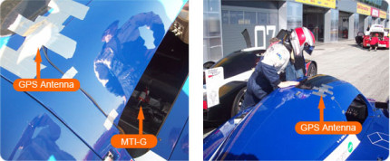
Figure 1: View of the GPS antenna (under the silver tape) and the MTi-G unit (68 grams) in the car

The MTi-G was mounted on top of a suitable vibration damper. An effective anti-vibration mount is very important to dampen the vibrations which the MTi-G unit is subjected to. Large vibrations could influence the accuracy of the measurements of the MTi-G.

Performance Bio racing LMP2
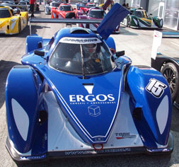	Chassis: Power: Torque: Gear-Box: Engine: Fuel:	Carbon 350 CV at 6.000 rpm 450 Nm at 4.500 rpm sequential 6 gears V6 4.0 L in longitudinal position at the rear Superethanol E85

Theory

The MTi-G can output 3D orientation, 3D position, 3D velocity and 3D calibrated inertial data such as accelerations and angular velocities in real time. By using this data, the following racing parameters can be derived from the MTi-G measurement unit:

Over steering and under steering

Over-steering and under-steering can be determined using the ‘DiffGyro’ data derived from the MTi-G data. ‘DiffGyro’ is the difference between the cornering rate of the trajectory and the vehicle rate of turn measured by the rate-gyroscope, Gz. Based on the sign of the ‘DiffGyro’ signal, we can analyze the steering behavior of the vehicle around the turns. The ‘DiffGyro’ can be calculated using the following formula:

The cornering rate can be derived from the position data or the velocity data. One way to compute cornering rate at a given sample point B is to consider the neighboring points A and C. There is an angle θ between the vectors AB and BC. The ‘Cornering rate’ = θ * freq / 2

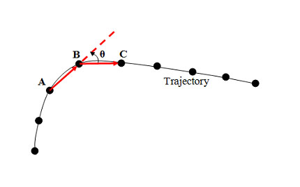
Figure 2: Calculating the cornering rate

Alternatively, if the velocity is divided by the radius and subtracted the vehicle rate of turn (Gz), the ‘DiffGyro’ can be calculated. With the DiffGyro, over- and under steering can be determined.

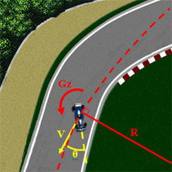
Figure 3: an over-steering situation. The rate of turn from the racing car is determined by the rate gyros, the cornering rate is calculated by the GPS values using the MTi-G as well. The ‘DiffGyro’ is less than zero or the rate of turn of the Gyro is higher than the cornering rate of the track. θ is the slip angle of the car at the center of gravity.

Slip Angle (figure 3)

The slip Angle (θ) is given at the GPS antenna location by the difference between the heading of the unit (aligned with the direction the car) and the tangent of the trajectory at the GPS antenna location (given by the velocity vector V). It is possible to calculate the slip angle at any points of the car with equations (VB = VA + BA ˄ W) because the MTI-G unit provides all the dynamics information to determine the velocity vector at a known distance from the GPS antenna location.

Radius of trajectory

When the cornering rate ‘W’ is known, the radius ‘R’ of the trajectory can be easily computed by R = Velocity (V) / cornering rate (W).

Accelerations and orientation behavior

The MTi-G outputs orientation data including roll and pitch. Therefore the raw data from the unit such as Ax, Ay and Gz can be easily corrected to the level plane. This correction has been applied in the computation of Ax, Ay and Gz as described.

Results

The following results were derived from the MTi-G data:

Over steering and under steering

The cornering rate and Gz were used to calculate the ‘DiffGyro’ value. Figure 4 displays a 2D plot of the ‘DiffGyro’ value, on one given lap. This gives an overview of the steering behavior of the driver and/or the car.

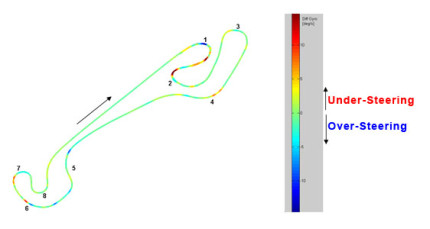
Figure 4: Overview of over-steering (to the blues) and under-steering (to the reds) at Nogaro circuit (south of France)

From this graph, we can quickly notice the following points:
Some under steering occurs at curve 4 which is a ‘brake tap and 100% throttle’ curve. Therefore, the driver should have a little bit of over-steer at the entrance (like at curve 5). Instead, the driver under-steers a little bit, which means that he brakes too early. There is a lot of under-steering at curve 2 which is the tightest one. This means that the driver does not manage to turn, probably because the car is not settled properly for this curve. It could be interesting to work with a different car set-up, to investigate how this influences the results.

Determining the optimum racing line

The ideal racing line can be derived from the brake and acceleration performance, and the driven trajectory as derived by using the MTi-G data. For this example, curve 1 from Figure 4 is particularly interesting to analyze.

Figure 5 shows the data acquisition plot (plotted exclusively from MTi-G data), with the corresponding points A, B and C on the track of curve 1. The X-axis displays the number of samples from A (which is directly related to time: sample rate is 200Hz). Figure 5 is a 2D plot of the acceleration profile of curve 1, where the driver tested two different trajectories (‘Inside-Outside’ and ‘Outside-Inside’) in two consecutives laps.

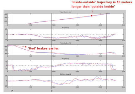
Figure 5: Data acquisition plot of curve 1. Red = ‘Inside-outside’ trajectory. Blue = ‘outside-inside’ trajectory.
The data sampling at 200 Hz of curve 1 can be used for calculation or to visualize as displayed in figure 6.

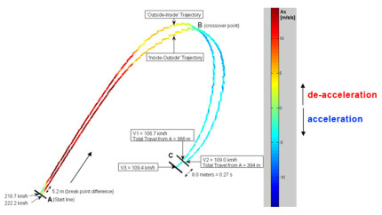
Figure 6: Zoom on two different trajectories at curve 1 with Ax indication (brake to the reds and acceleration to the blues)
Concluded from the graph is that the ‘inside-outside’ trajectory quicker is than the ‘outside-inside’, which saves the driver 0,27 seconds.

With the MTi-G data it is possible to calculate the brake point and the exact distance between the two brake points: 5.2 meters (‘Outside-Inside’ Trajectory had to brake earlier, firstly to catch the inside of the corner and secondly because the entry speed at point A is a bit higher). The MTi-G time corresponding to the plot of the two trajectories is exactly the same. Therefore we can immediately deduce that ‘Inside-Outside’ trajectory is quicker than ‘Outside-Inside’ trajectory because in the same time the driver traveled more (8.0 meters). The driver saves 0.27 seconds if taking the ‘inside-outside’ line. ‘Inside-Outside’ Trajectory is more likely to be a formula trajectory with a ‘V’ whereas the second is smoother at the inner of the curve. This can be checked with the computation of the minimum of the radius of the trajectory of the curve (around point B): 37.7 meters compared to 40.4 meters.

If we look purely at the data acquisition plot of Figure 6, the velocity of the ‘Inside-Outside’ trajectory at point C looks somewhat higher. But this is because it is function of time: at point C there is a 0.27 s of delay which corresponds to 8.0 meters. Therefore at point C on figure 6, V3 = 109.4 km/h is fmeasured instead of V2 = 106.7 km/h (see figure 5). It is then interesting to note that the ‘Outside-Inside’ trajectory enables the curve to be taken faster at point B and also to exit this curve faster (109.0 km/h compared to 106.7 km/h). This is because on that part of the track, there is more grip. If we look at the over steering plot, we can see that the over steering phase during the ‘V’ (negative DiffGyro phase showed by the black ellipses in figure 5) is higher and quicker for the ‘Inside-Outside’ trajectory, hence the ‘V’ enables earlier acceleration ,as figure 5 clearly shows at B, and hence the gap between the two velocities starts reducing from the start of the ellipse.

Conclusion

The MTi-G miniature AHRS has been tested within a Bio-racing car at the Nogaro circuit (south of France). The MTi-G provided data to determine the optimum racing line, brake / acceleration profiles, over-steering and under-steering behavior, slip angle, radius of the trajectory and the velocity profile on the track.

About an order of magnitude less in terms of size, power consumption and costs compared to the high end measurement systems, the MTi-G is a low entry barrier for gaining excellent data for analyzing and improving racing applications.

For more information about Xsens MTi-G, please visit our MTi-G-710 productpage or contact sales@xsens.com